Cycling in London is not the most pleasurable ride, one could say for the drivers’ attitude against cyclists, but mostly because I hate riding in the rain. And, you know, rain-wise London is nowhere as bad as people like to complain, but nevertheless it’s bad.

I started commuting to and from work with my bike, but it seems that it’s always raining, or worse that it’s not raining but the bike is in the other place because I failed to bring it with me last time. Are these feelings real?

Let us formalize the problem: suppose that \( X\% \) of the times I need to commute it’s raining; then, what ratio of my commutes are done cycling? As mentioned before, the bike could be misplaced, hence it cannot be more than \( X\% \). We can construct an evolving model of the situation after every night: we can consider the probability that after the \( n \)-th night the bike is at home and name it \( h_n \), and symmetrically \( w_n = 1 - h_n \) will be the probability that the bike is at work.

At the beginning, \( h_0 = 1 \) because the initial state is with the bike at home. After the first day, the bike is at home again either because we rode forth and back (probability \( (1 - X)^2 \), that is, it was not raining both in the morning and in the evening), or because the bike never left home (probability \( X \), since it is enough that on the morning it was raining). In symbols, \( h_1 = (1 - X)^2 + X = 1 - X + X^2 \), and of course \( w_1 = 1 - h_1 = X - X^2 \).

For the following days, \( h_n \) will have two components: one assuming that the bike was at home the previous night (similar to what we did for computing \( h_1 \)), and another if we assume the bike at work. In this latter case, the probability that it was at home the following night are just \( (1 - X) \): whatever happens in the morning is not relevant, therefore it is enough being able to come back in the evening. Putting all together, we get \( h_n = h_{n-1} (1 - X + X^2) + w_{n-1} (1 - X) = h_{n-1}(1 - X + X^2) + (1 - h_{n-1})(1 - X) \), which is \( 1 - X + h_{n-1}X^2 \).

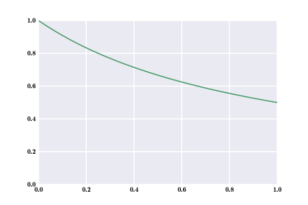
Solving sequences like this was actually one of the first topic I learned as a math student exactly ten years ago. It is quite simple: one computes the first values of the sequence to get an idea of what is happening; in our case, with an example value of \( 50\% \) for \( X \), the first few values are \( 1 \), \( 0.75 \), \( 0.6875 \), \( 0.671875 \), \( 0.6679875 \), \( \dots \). There is already a good news, as we may conjecture (and easily prove) that the sequence is always decreasing; on the other hand, being a probability, it is bounded between \( 0 \) and \( 1 \). And there is an easy theorem saying that non-increasing, lower bounded sequence admit a limit. To find the limit, just solve the equation \( h_{\infty} = 1 - X + h_{\infty}X^2 \), that is, \( h_{\infty} = \frac{1}{1 + X} \), or \( h_{\infty} = 2/3 \) for \( X = 50\% \) (as we could guess from the first few elements of the sequence).

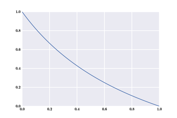
As for the ratio of commutes by bike among all commutes, it is now easy to compute: the ratio for the morning and for the evening must be equal, because after a short while the situation evolves in a completely symmetrical fashion. Cycling in the morning happens exactly if the bike is at home and it is not raining, hence it happens with probabily \( h_{\infty} \cdot (1-X) = \frac{1-X}{1+X} \) (in our example, one third of the times).The graphs showing how this ratio changes with the rain probability are not very exciting, they just show an expected decrease of the ratio as the probability of rain increases, slightly sublinear (we saw that for \( X = 50\% \) the ratio is \( 1/3 \)).